QIRX SDR

Calibrate your RTL-SDR in 15 Seconds (Seconds, not Minutes)
Part III: Improving DAB
A Tutorial by Clem, DF9GI
This third and last part of the "Calibration" tutorial series will explain why it is beneficial for the DAB reception to correct not only the frequency error of our ultra-cheap hardware, but also its sampling rate. Before going into this, we'll have a short look at the anatomy of our DAB spectrum and understand why it is necessary to observe the DAB signal at exactly its generated frequency.
Orthogonality
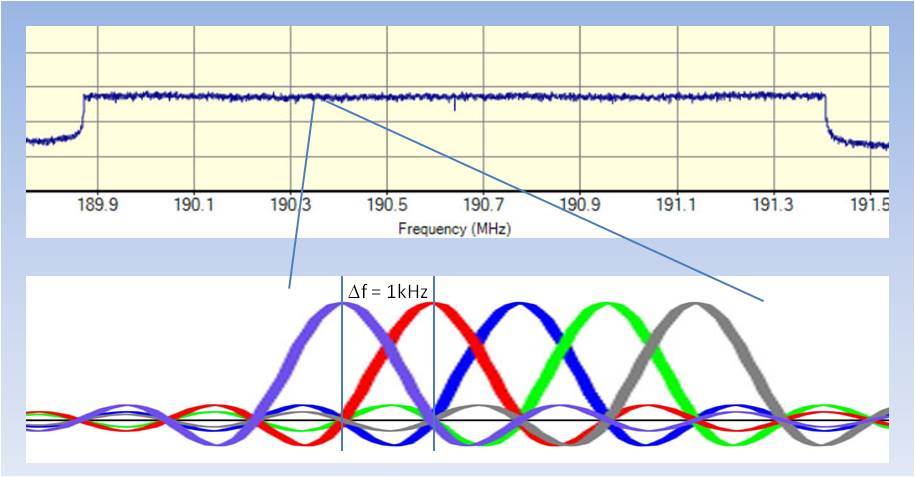
The upper part of the picture shows the well-known spectrum of a decent DAB signal. The active DAB part spans a frequency range
of 1537kHz. The information is contained in 1536 carriers (the central carrier is suppressed), with a distance of 1kHz to each other.
For illustration, the lower part of the picture shows an extract of 5kHz, and the shape of the single carriers. Don't worry about the carrier shape, we'll see
in a moment where it comes from.
You probably know that a DAB signal is constructed according to the OFDM scheme (OFDM = Orthogonal Frequency-Division Multiplexing).
The letter which interests us here is the "O" of OFDM. What means "orthogonal" and how is it connected to our frequency calibration?
The main principle is easy to understand. It simply means that neighboring carriers don't influence each other. At first glance,
this is surprising, because obviously the carriers strongly overlap, as you can see in the lower part of the picture. And now
we already are in the very center of our problem, which consists in the fact that we have to tune the DAB receiver with a very high
accuracy to the frequency of the transmitter.
Please have a look at the colored curves. If we manage to tune our receiver exactly at the transmitter's frequency, then
we observe our signal exactly at the peak of each colored curve. And here comes the trick: Consider - as an example - the left (violet) carrier.
The amplitudes of all of its neighbors (e.g. the red one) are zero at the violet peak. Zero amplitude = no influence from those
carriers = Orthogonality. The same happens with all other carriers. On the peak of each of them, all others are orthogonal (= zero amplitude).
Very nice and really tricky. By the way, DAB has been the first standard based on
OFDM (1995). Today, everybody does it, DSL, DVB-T2, WiFi, LTE, to name only a few. A really powerful principle.
Let's see how it works in practice. To demonstrate I'll mis-align
the receiver intentionally and see what happens. Even better: DIY! How? In QIRX, just uncheck
in the "Synchronization" box the item "Auto Fine Frequ.".
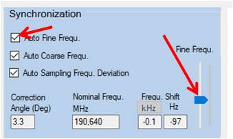 Now you are able to manually fine-tune the frequency with the "Fine Freq." slider
being located on the right side of the box.
Now you are able to manually fine-tune the frequency with the "Fine Freq." slider
being located on the right side of the box.
Inter Carrier Interference
The magnitude (better: power) of our spectrum shows us its quality, the signal strength, SNR, multipath etc., but it does NOT show
us the information the carriers are transporting, their payload. This is contained in the phase of the carriers, and is visualized in the constellation spectrum.
We are interested in how much the constellation of a good signal deteriorates if we tune the center frequency off its nominal, calibrated value.
This "deterioration" is called "Inter Carrier Interference" (ICI) and is shown in the next picture.
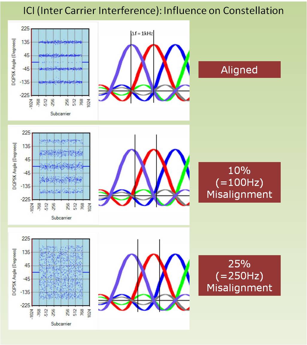
These pictures show very clearly that it is necessary to precisely compensate the center frequency offset - causing ICI - of
our receiver. Even a moderate ICI of 100Hz ruines the constellation completely, as it shifts the angles between
two quadrants, thus making a proper decoding impossible. (QIRX has a control loop shifting the constellation back into the right
place, which was intended for a hardware-based frequency compensation, having been omitted for some reasons. The loop, however, is
still in action).
The second effect of ICI is a noise-like degradation of the constellation, stemming from the - now nonzero - influence
of the neighboring carriers, i.e. the destroyed orthogonality. Applying a misalignment of 250Hz, even the regualrity of the
constellation cannot be recognized any more, it looks like random noise.
Carrier Shape
You noticed the shape of the carriers, shown - for illustration - in various colors? The curve is a sin(x)/x, usually
called sinc. This sinc-shaped curve is the Fourier Transform of a simple rectangular time function, as shown in the picture.
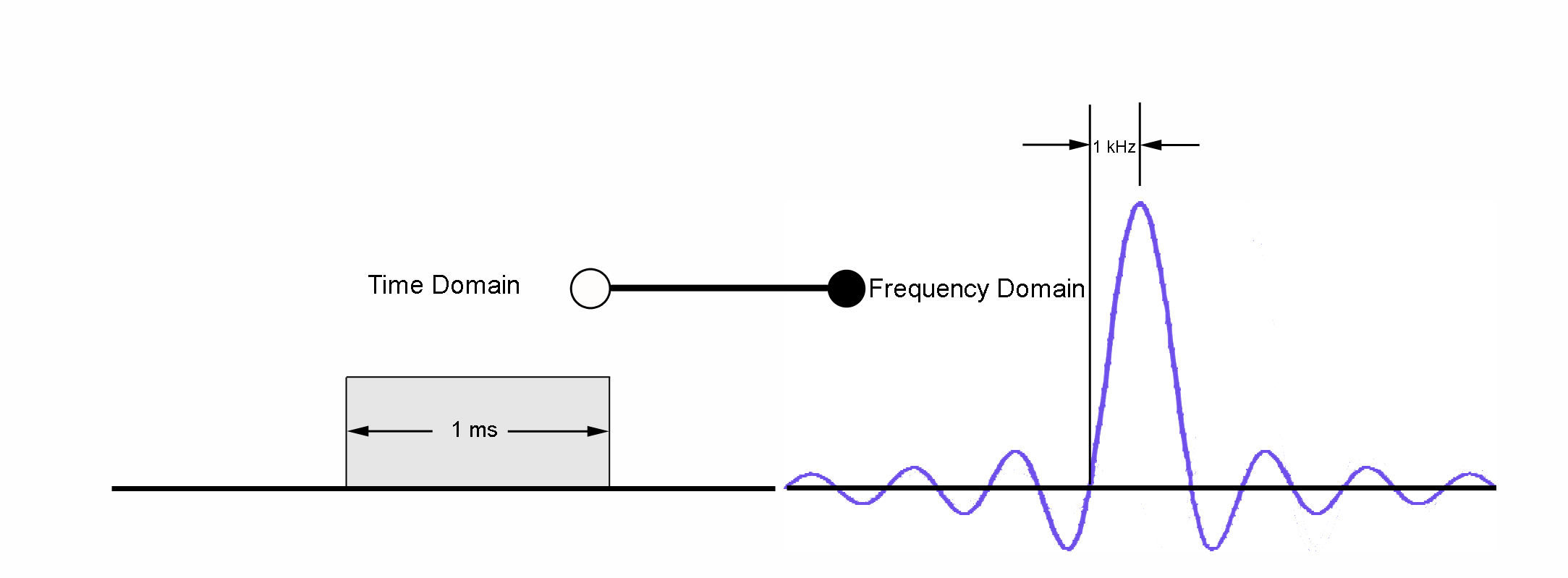
What is done by the transmitting side is - in DAB - a generation of all 2048 carriers (1536 carrying the payload)
in the time of 1Millisecond. This is serialized with the consequence that our receivers have to process 2048*1000 I/Q samples every second.
The transmitter permanently generates for every carrier a sine of the duration on 1ms, the sine having the frequency of the carrier.
This limited duration means that this sine is multiplied by a rectangle. This is in time domain. In frequency domain, meaning after application
of a FFT, such a signal transforms to the shown sinc function , centered at the frequency of the sine.
In case you should be interested to dive deeper into this or many other items of signal processing, I can highly recommend
the website "wirelesspi.com" of Qasim Chaudhari. In particular, Qasim shows a tutorial
called A Beginner’s Guide to OFDM, where he is explaining
many fundamental details of OFDM in a very understandable way.
Qasim also is the creator of the nice colored
picture showing the orthogonal carriers, and has kindly given his approval to use it here.
Sampling Rate
Now let us deal with the influence of sampling rate errors on the received and decoded signals. To start, have a look at the signal
we are going to investigate and manipulate.
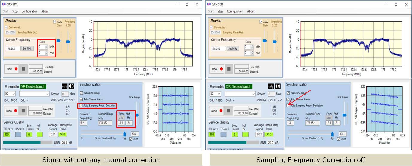
The left picture shows a strong signal with two notches due to multipath. All manual corrections like ppm value and Delta kHz are off,
the Auto Sampling Frequency Correction is on. Everything is done automatically.
The right picture shows the identical signal, with one difference:
The "Auto Sampling Frequency Correction" is switched off. The effect is clearly visible in the constellation: The oblique straight lines indicate
a linear error of the DQPSK angles depending on the subcarrier. The error angle seems to be proportional to the subcarrier number. Nevertheless, all bits are still in their correct quadrant, because there is little
scattering in this strong signal.
In the next step we'll artificially create a really bad RTL-SDR receiver, to find out the limit when decoding
will start to deteriorate due to
a sampling rate error. To exclude effects based on the center frequency error, we will let the hardware compensate it.
As a consequence, we'll apply a suitable
center frequency offset, and step-by-step increase the sampling rate error by applying an increasingly wrong ppm value. But first let us
do some cross-checks to see whether the numbers we are going to enter are reasonable.
As we have seen in the first part, the dongle I am using for this tutorial
has a sampling frequency error of about 46ppm (the same
value as the center frequency error, which we will compensate separately, as mentioned).
The total ppm error calculates by adding the inherent dongle error of 46 ppm to the additionally value (sign inverted) entered
into the "ppm" field in the "Device" box.
Please have a look at the next picture.
-
Cross-Check: Center Frequency correction
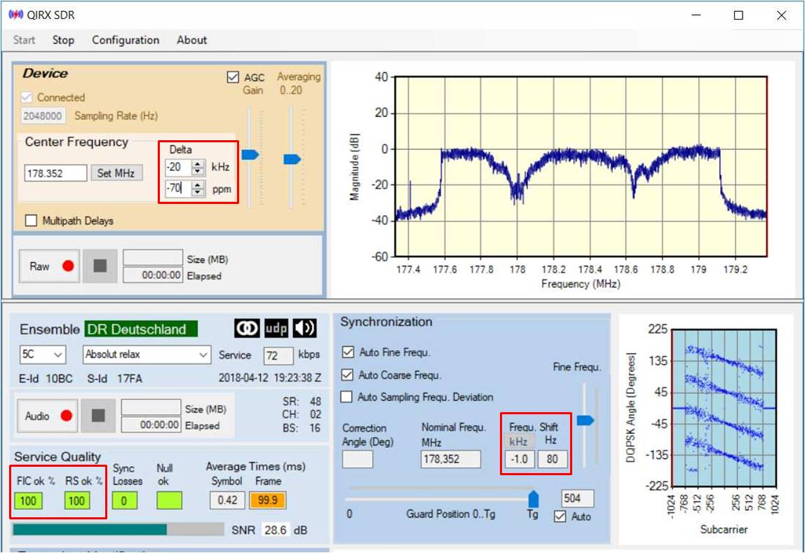
For instance, by entering -70ppm into this field (see picture below) we get total ppm error of -46-70= -116ppm.
We can cross-check the correctness of this value by calculating the center-frequency error of -116ppm. At 178.352MHz, -116ppm correspond
to -20.7kHz, meaning we must change the center frequency by this value for a correction by hardware. Inspecting the picture below, we added -20kHz to the center frequency,
leaving a residual -1kHz for correction by the software. This is the value we find in the "Frequ.Shift" field (rightmost red rectangle). Cross-check successful.
-
Cross-Check: Sampling Rate correction
By entering -70 into the "ppm" field, we can also assume a sampling rate
error of -116ppm, corresponding to -238Hz, because -again - the ppm value sent to the hardware corrects the sampling rate as well.
The software measures this value, and uses it for the compensation of the error. Although this value does not
show up on the GUI, for verification we can run the software with a debugger, set a breakpoint in the proper place, and read the
value. In doing this, we get - software calculated - values between 236 and 240 Hz, changing a little between different DAB frames (the
calculation and correction in the software always takes place between frames). Sampling Rate cross-check succeeded.
-
Sampling Error: (-46-70)ppm = -116ppm
As described above, entering a value of -70 into the "ppm" field will give us a sampling rate error of -116ppm, because
the dongle shows an inherent error of 46ppm. The result without a compensation of this error is shown in the
above picture. We observe the following effects:
-
Constellation Angle Error
The DQPSK bits show an error proportional to their subcarrier. In the center of the constellation (Subcarrier around zero),
the bits still sit on their proper place. The deviation increases linearly with the subcarrier. On the highest subcarriers,
the angles already start to "wrap-around".
-
Noise-like degradation
On the higher subcarriers, the bits show an increased scattering around their center values. This looks similar to
the Inter Carrier Interference (ICI) we observed in the investigation of the Orthogonality (see above).
-
Perfect Decoding
Despite the fact that the bits on the higher subcarriers sit far off their correct position, the
Service Quality still is 100% (lower left rectangle).
The Reed-Solomon error corrector still has nothing to do, as 100% of the superframes are going
without correction. We attribute this behaviour to the efficient work of the Viterbi decoder, not shown on the GUI.
-
Confirmation of the Theory
Theorists have long predicted the shown behaviour. In [1] the following effects are stated due
to a sampling rate error of OFDM systems:
- Amplitude Reduction
- ICI
- Phase Shift proportional to the subcarrier
Our measurements are in-line with these predictions and -at least- confirm the ICI and the phase shift. We did not try any measurement of the predicted
amplitude reduction.
-
Gain Reduction
Now let us deteriorate the situation further by reducing the gain, simulating a rather weak signal with its
strong multipath notches. Again, in both cases the center frequency offset is corrected by the hardware, the software
corrected "Frequ.Shift" being zero.
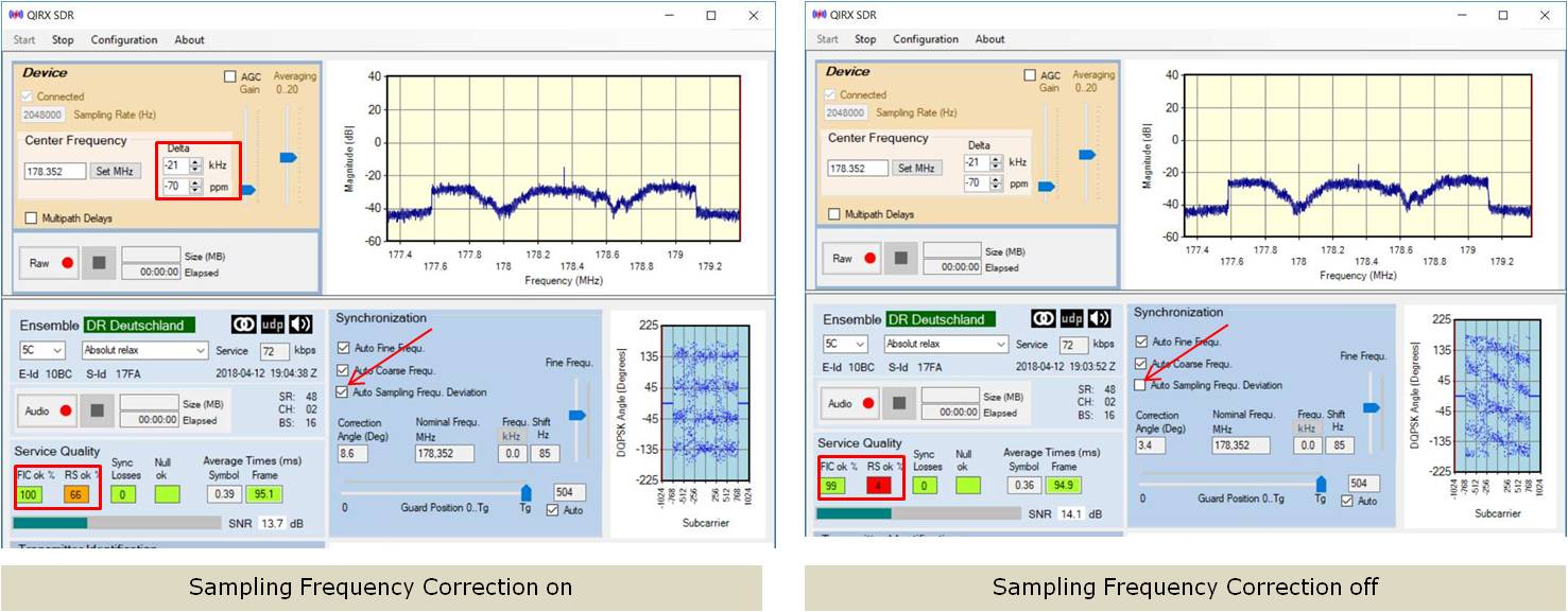
The left picture - with sampling frequency corrected - still has 100% of the "Fast Information Channel (FIC)" detected, but the
Reed-Solomon starts to work, only 66% of the DAB+ superframes passed without correction (lower left rectangle).
The quality of the sampling frequency error correction manifests itself by showing horizontally aligned angle bits. Due to the
various error correction mechanisms, the signal is still perfectly readable.
This contrasts to the right picture, its only difference being the switched-off sampling error correction.
The Reed-Solomon (RS) practically has to correct every frame. However, with respect to the RS error corrector it must be mentioned
that the shown values of the pictures are snapshots. The RS-values show a rather wide range indicating a trend of the quality.
This signal is still audible with interruptions. This is in no way surprising looking at the constellation. Clearly, for
such a signal the sampling rate error correction is mandatory for a clean reception.
-
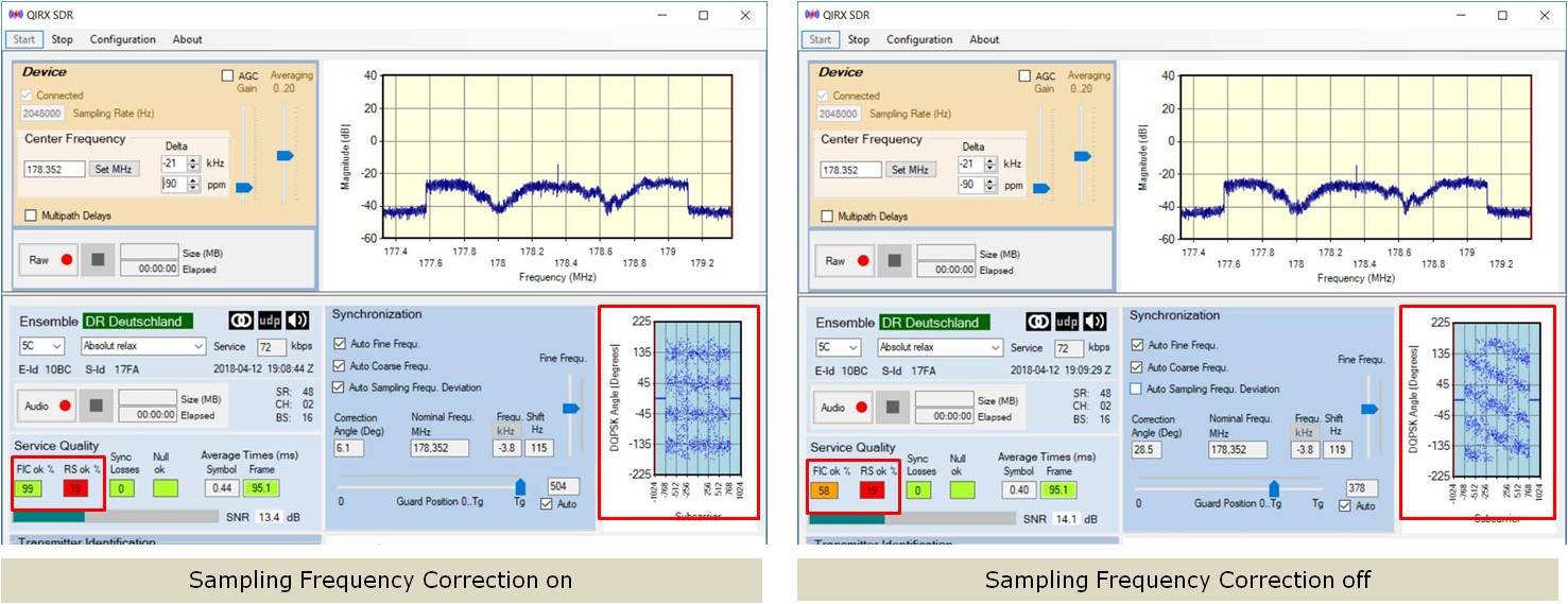
Sampling Error: (-46-90)ppm = -136ppm
To terminate this series, the last two pictures show the same scenario, but with a ppm induced error of -46-90=-136ppm.
The left signal having the sampling rate error corrected is well readable and similar to the last one (with correction).
The signal without
the sampling rate error correction is unreadable.
-
Conclusions
-
Receiver
Correcting the sampling rate error allows for a use of receivers with large tolerances. The experiments
shown here demonstrate the successful use of a receiver having a sampling rate error of -135ppm, by applying
a software-based correction. Without correction, a hardware with such a large clock error is not DAB-usable any more.
-
Hardware-Based Correction
To use the benefits of a corrected sampling rate, the easiest way would perhaps be to program the hardware with
the sampling rate error compensation obtained by the calibration of the receiver (see previous parts of this tut).
The measured "ppm" deviation can be used for the simultaneous correction of the center frequency and
the sampling rate error. QIRX offers the possibility to store the last used value and applies it on startup.
-
"Normal" Hardware and Signals
The experiments show that for DAB the use of receivers with "usual" clock tolerances of about 50ppm does not require
the correction of the sampling rate error.
-
Measurement Principle
In the software, the sampling rate error is obtained by measuring the Channel Impulse Response (CIR). In a nutshell, this
is a correlation-based measurement of the start-time of the Phase Reference Symbol (PRS) at the beginning of each frame, after the Null
Symbol. The deviation of the PRS start time from its nominal value (= Tg = 504 samples in DAB Mode I) can be used as a precise
measure of the sampling rate error.
This timing error can be converted into a frequency
error and into an angle error. Before the decoding of the DQPSK bits, that angle is multiplied with its subcarrier
number and used as a correction. In this way, the oblique constellation lines indicating a sampling error are converted into
horizontal lines compensating the error.
By the way, in a multipath environment the CIR measurement produces more than one peak
which can be evaluated to estimate the delay times of different signal paths, serving as a guide how to position the FFT-Window. This,
however, would be a different story.
For instance, by entering -70ppm into this field (see picture below) we get total ppm error of -46-70= -116ppm. We can cross-check the correctness of this value by calculating the center-frequency error of -116ppm. At 178.352MHz, -116ppm correspond to -20.7kHz, meaning we must change the center frequency by this value for a correction by hardware. Inspecting the picture below, we added -20kHz to the center frequency, leaving a residual -1kHz for correction by the software. This is the value we find in the "Frequ.Shift" field (rightmost red rectangle). Cross-check successful.
By entering -70 into the "ppm" field, we can also assume a sampling rate error of -116ppm, corresponding to -238Hz, because -again - the ppm value sent to the hardware corrects the sampling rate as well. The software measures this value, and uses it for the compensation of the error. Although this value does not show up on the GUI, for verification we can run the software with a debugger, set a breakpoint in the proper place, and read the value. In doing this, we get - software calculated - values between 236 and 240 Hz, changing a little between different DAB frames (the calculation and correction in the software always takes place between frames). Sampling Rate cross-check succeeded.
As described above, entering a value of -70 into the "ppm" field will give us a sampling rate error of -116ppm, because the dongle shows an inherent error of 46ppm. The result without a compensation of this error is shown in the above picture. We observe the following effects:
-
Constellation Angle Error
The DQPSK bits show an error proportional to their subcarrier. In the center of the constellation (Subcarrier around zero), the bits still sit on their proper place. The deviation increases linearly with the subcarrier. On the highest subcarriers, the angles already start to "wrap-around". -
Noise-like degradation
On the higher subcarriers, the bits show an increased scattering around their center values. This looks similar to the Inter Carrier Interference (ICI) we observed in the investigation of the Orthogonality (see above). -
Perfect Decoding
Despite the fact that the bits on the higher subcarriers sit far off their correct position, the Service Quality still is 100% (lower left rectangle). The Reed-Solomon error corrector still has nothing to do, as 100% of the superframes are going without correction. We attribute this behaviour to the efficient work of the Viterbi decoder, not shown on the GUI. -
Confirmation of the Theory
Theorists have long predicted the shown behaviour. In [1] the following effects are stated due to a sampling rate error of OFDM systems:
- Amplitude Reduction
- ICI
- Phase Shift proportional to the subcarrier
Our measurements are in-line with these predictions and -at least- confirm the ICI and the phase shift. We did not try any measurement of the predicted amplitude reduction.
Now let us deteriorate the situation further by reducing the gain, simulating a rather weak signal with its
strong multipath notches. Again, in both cases the center frequency offset is corrected by the hardware, the software
corrected "Frequ.Shift" being zero.
The left picture - with sampling frequency corrected - still has 100% of the "Fast Information Channel (FIC)" detected, but the Reed-Solomon starts to work, only 66% of the DAB+ superframes passed without correction (lower left rectangle).
The quality of the sampling frequency error correction manifests itself by showing horizontally aligned angle bits. Due to the various error correction mechanisms, the signal is still perfectly readable.
This contrasts to the right picture, its only difference being the switched-off sampling error correction. The Reed-Solomon (RS) practically has to correct every frame. However, with respect to the RS error corrector it must be mentioned that the shown values of the pictures are snapshots. The RS-values show a rather wide range indicating a trend of the quality. This signal is still audible with interruptions. This is in no way surprising looking at the constellation. Clearly, for such a signal the sampling rate error correction is mandatory for a clean reception.
-
Sampling Error: (-46-90)ppm = -136ppm
To terminate this series, the last two pictures show the same scenario, but with a ppm induced error of -46-90=-136ppm. The left signal having the sampling rate error corrected is well readable and similar to the last one (with correction). The signal without the sampling rate error correction is unreadable.
-
Conclusions
-
Measurement Principle
In the software, the sampling rate error is obtained by measuring the Channel Impulse Response (CIR). In a nutshell, this is a correlation-based measurement of the start-time of the Phase Reference Symbol (PRS) at the beginning of each frame, after the Null Symbol. The deviation of the PRS start time from its nominal value (= Tg = 504 samples in DAB Mode I) can be used as a precise measure of the sampling rate error. This timing error can be converted into a frequency error and into an angle error. Before the decoding of the DQPSK bits, that angle is multiplied with its subcarrier number and used as a correction. In this way, the oblique constellation lines indicating a sampling error are converted into horizontal lines compensating the error.
By the way, in a multipath environment the CIR measurement produces more than one peak which can be evaluated to estimate the delay times of different signal paths, serving as a guide how to position the FFT-Window. This, however, would be a different story.
The left picture - with sampling frequency corrected - still has 100% of the "Fast Information Channel (FIC)" detected, but the Reed-Solomon starts to work, only 66% of the DAB+ superframes passed without correction (lower left rectangle).
The quality of the sampling frequency error correction manifests itself by showing horizontally aligned angle bits. Due to the various error correction mechanisms, the signal is still perfectly readable.
This contrasts to the right picture, its only difference being the switched-off sampling error correction. The Reed-Solomon (RS) practically has to correct every frame. However, with respect to the RS error corrector it must be mentioned that the shown values of the pictures are snapshots. The RS-values show a rather wide range indicating a trend of the quality. This signal is still audible with interruptions. This is in no way surprising looking at the constellation. Clearly, for such a signal the sampling rate error correction is mandatory for a clean reception.
To terminate this series, the last two pictures show the same scenario, but with a ppm induced error of -46-90=-136ppm. The left signal having the sampling rate error corrected is well readable and similar to the last one (with correction). The signal without the sampling rate error correction is unreadable.
-
Receiver
Correcting the sampling rate error allows for a use of receivers with large tolerances. The experiments shown here demonstrate the successful use of a receiver having a sampling rate error of -135ppm, by applying a software-based correction. Without correction, a hardware with such a large clock error is not DAB-usable any more. -
Hardware-Based Correction
To use the benefits of a corrected sampling rate, the easiest way would perhaps be to program the hardware with the sampling rate error compensation obtained by the calibration of the receiver (see previous parts of this tut). The measured "ppm" deviation can be used for the simultaneous correction of the center frequency and the sampling rate error. QIRX offers the possibility to store the last used value and applies it on startup. -
"Normal" Hardware and Signals
The experiments show that for DAB the use of receivers with "usual" clock tolerances of about 50ppm does not require the correction of the sampling rate error.
In the software, the sampling rate error is obtained by measuring the Channel Impulse Response (CIR). In a nutshell, this is a correlation-based measurement of the start-time of the Phase Reference Symbol (PRS) at the beginning of each frame, after the Null Symbol. The deviation of the PRS start time from its nominal value (= Tg = 504 samples in DAB Mode I) can be used as a precise measure of the sampling rate error. This timing error can be converted into a frequency error and into an angle error. Before the decoding of the DQPSK bits, that angle is multiplied with its subcarrier number and used as a correction. In this way, the oblique constellation lines indicating a sampling error are converted into horizontal lines compensating the error.
By the way, in a multipath environment the CIR measurement produces more than one peak which can be evaluated to estimate the delay times of different signal paths, serving as a guide how to position the FFT-Window. This, however, would be a different story.
Reference: [1] Maja Sliskovic: Sampling Frequency Offset Estimation and Correction in OFDM Systems, Electronics, Circuits and Systems, 2001. ICECS 2001. As always with IEEE: costly!
Home